Introduction to Neural Networks
A neural network is a computational model inspired by the way biological neural networks in the human brain process information. It consists of layers of neurons, each neuron performing a mathematical operation. The main goal of a neural network is to learn from the data and make accurate predictions.
Also called feedforward neural networks, or multilayer perceptrons (MLPs), are the quitessential deep learning models.
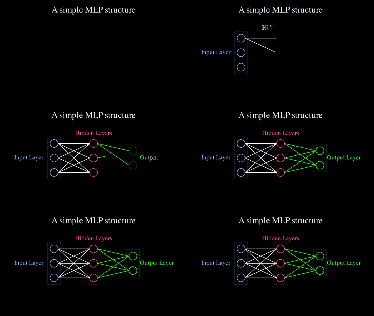
In its simplest form, a neural network has three types of layers:
- Input Layer: Where data enters the network.
- Hidden Layers: Where data is processed with mathematical transformations.
- Output Layer: Where the final prediction or classification is made.
Below you can see a very simple structure of how an MLP is:

Neurons and Layers
Each neuron (circles in the gif above) receives an input, performs a weighted sum, and applies an activation function. Mathematically, a neuron in layer \( l \) can be described as:
$$ z^{(l)} = W^{(l)} \cdot a^{(l-1)} + b^{(l)} $$
where:
- \( W^{(l)} \): Weight matrix for layer \( l \).
- \( a^{(l-1)} \): Activation from the previous layer.
- \( b^{(l)} \): Bias vector for layer \( l \).
Let's see a simple visualization of how a neuron works. Of course this visualization is not entirely correct with respect to the actual mathematical operations that take place in a neuron, but it gives a good idea of what's happening. Basically, the neuron takes an input (an object with a color), multiplies it by a weight, and adds a bias.

However, if you're already familiar with how neural networks work, you can definitely point out something missing in the previous animation. What is it? The Activation function!
The output of each neuron is passed through an activation function like ReLU or Sigmoid. That is, given the output of a neuron \( z^{(l)} \), the activation function is applied to it to get the output \( a^{(l)} \):
$$ a^{(l)} = f(z^{(l)}) $$
where \( f \) is the activation function.
For instance we can have different activation functions defined by the following equations:
- Sigmoid: \( f(x) = \frac{1}{1 + e^{-x}} \)
- ReLU: \( f(x) = \max(0, x) \)
- Tanh: \( f(x) = \frac{e^x - e^{-x}}{e^x + e^{-x}} \)
Forward Propagation
In forward propagation, data passes through each layer, transforming inputs into outputs through matrix multiplication, bias addition, and activation functions. For a simple feedforward network:
$$ a^{(1)} = f(W^{(1)} \cdot X + b^{(1)}) $$
The forward pass continues through each hidden layer until it reaches the output layer. If the network has multiple hidden layers, the process can be generalized as:
$$ a^{(l+1)} = f(W^{(l+1)} \cdot a^{(l)} + b^{(l+1)}) $$
Loss Function
The loss function quantifies how well the network's predictions match the true values. For regression tasks, the Mean Squared Error (MSE) is commonly used:
$$ L = \frac{1}{N} \sum_{i=1}^{N} (y_i - \hat{y}_i)^2 $$
where:
- \( y_i \) is the true value for the \( i^{th} \) training example.
- \( \hat{y}_i \) is the predicted value.
- \( N \) is the number of training examples.
In classification tasks, the cross-entropy loss is often used:
$$ L = - \sum_{i=1}^{N} y_i \log(\hat{y}_i) $$
Backpropagation and the Chain Rule
Backpropagation is used to compute gradients of the loss function with respect to each weight in the network. It applies the chain rule of calculus to propagate the error backward through the network. The gradient of the loss with respect to the weight \( W \) is:
$$ \frac{\partial L}{\partial W} = \frac{\partial L}{\partial \hat{Y}} \cdot \frac{\partial \hat{Y}}{\partial Z} \cdot \frac{\partial Z}{\partial W} $$
This process allows the network to adjust weights in order to minimize the error.
Gradient Descent
Gradient descent is an optimization technique used to minimize the loss function by updating the weights in the direction of the negative gradient. The weight update rule is:
$$ W^{(t+1)} = W^{(t)} - \eta \nabla_W L $$
where:
- \( W^{(t)} \) is the weight at step \( t \).
- \( \eta \) is the learning rate.
- \( \nabla_W L \) is the gradient of the loss with respect to the weights.
Regularization and Overfitting
Regularization techniques help prevent overfitting, where a model performs well on training data but poorly on unseen data. One common regularization technique is L2 regularization, which adds a penalty term to the loss function:
$$ L_{total} = L + \lambda \sum ||W||^2 $$
where \( \lambda \) controls the strength of the regularization, and \( W \) is the weight matrix.
Types of Neural Networks
There are various types of neural networks, each suited to different tasks:
- Feedforward Neural Networks (FNN): The simplest form of neural networks where information moves in one direction—from input to output.
- Convolutional Neural Networks (CNN): Primarily used for image recognition, CNNs apply convolutional layers to detect features in input images.
- Recurrent Neural Networks (RNN): Used for sequential data such as time series or natural language, RNNs maintain information across steps in the sequence.
- Long Short-Term Memory (LSTM): A specialized RNN that handles long-range dependencies by remembering important information over extended sequences.
- Autoencoders: Used for data compression and feature learning, they encode input into a lower-dimensional space and then reconstruct the output.