Introduction to Causal Inference
Causal inference is the process of determining whether one variable causes another variable to change. It is a fundamental concept in statistics and machine learning, and it is used to understand the relationships between variables in a dataset.
But before we can learn the fundamentals of causal inference let's understand what is Randomized Controlled Tests (RCTs) are.
Randomized Controlled Tests (RCTs)
A RCTs is an experiment where the subjects are randomly assigned to different groups, and the effect of the treatment is observed.
But what's is a treatment?
In the context of causal inference, a treatment refers to an intervention or an action that is intentionally applied to a group of subjects to observe its effect on an outcome. Here are some key aspects of a treatment:
- Intentional application: The treatment is deliberately applied to a group of subjects, as opposed to a natural occurrence.
- Manipulation of a variable: The treatment involves changing the value of a specific variable to observe its effect on the outcome.
- Comparison to a control group: The effect of the treatment is compared to a control group that does not receive the treatment.
- Goal of causal inference: The primary goal is to establish a cause-and-effect relationship between the treatment and the outcome.
Example: Evaluating the Effectiveness of a New Drug
Objective: Determine whether a new drug is effective in lowering blood pressure.
Step 1: Define the Treatment and Outcome
- Treatment: The new drug.
- Outcome: Reduction in blood pressure.
Step 2: Random Assignment
Randomization: Randomly assign participants into two groups:
- Treatment Group: Receives the new drug.
- Control Group: Receives a placebo (no active drug).
Step 3: Conduct the Experiment
Implementation: Administer the drug to the treatment group and the placebo to the control group over a specified period.
Blinding: Ensure that participants and researchers do not know who receives the treatment or placebo to prevent bias (double-blind study).
Step 4: Measure the Outcome
Data Collection: Measure blood pressure in both groups at the end of the study period.
Step 5: Analyze the Results
Comparison: Compare the average blood pressure reduction between the treatment and control groups.
Statistical Analysis: Use statistical tests (e.g., t-test) to determine if the difference in blood pressure reduction is statistically significant.
Step 6: Draw Conclusions
Causal Inference: If the treatment group shows a significantly greater reduction in blood pressure compared to the control group, infer that the new drug is effective in lowering blood pressure.
Consider Confounders: Ensure that randomization has effectively controlled for confounding variables, which could otherwise bias the results.
Step 7: Report Findings
Documentation: Report the methodology, statistical analysis, and conclusions in a scientific manner, ensuring transparency and reproducibility.
Example of Confounders
In our study evaluating the effectiveness of a new drug in lowering blood pressure, a potential confounder could be the participants' baseline physical activity levels. If participants in the treatment group are more physically active than those in the control group, the observed reduction in blood pressure might be due to their higher activity levels rather than the drug itself.
This could lead to an incorrect conclusion that the drug is effective when, in fact, the difference is due to the confounding effect of physical activity. To address this, researchers should ensure proper randomization, stratification, or statistical adjustment to control for such confounders.
Causal Inference Challenges
Causal inference is a powerful tool for understanding cause-and-effect relationships, but it comes with several challenges that researchers must address to ensure valid conclusions. Here are some of the key challenges:
Confounders
Confounders are variables that are related to both the treatment and the outcome, potentially leading to biased results if not properly controlled. For example, in a drug effectiveness study, participants' baseline physical activity levels could confound the results. Strategies to address confounders include:
- Randomization: Proper randomization can help distribute confounders evenly across treatment and control groups.
- Statistical Adjustment: Use statistical methods, such as multivariable regression, to adjust for confounders in the analysis.
- Machine Learning Techniques: Techniques like propensity score matching can be used to balance confounders between groups.
Selection Bias
Selection bias occurs when the participants selected for a study are not representative of the target population, leading to skewed results. This can happen if certain groups are overrepresented or underrepresented in the study, or if the study does not include a representative sample of the population. Strategies to address selection bias include:
- Matching: Matching techniques can be used to balance the characteristics of the participants in the study.
- Propensity Score Matching: Propensity score matching can be used to balance the characteristics of the participants in the study.
Counterfactuals
Counterfactuals are hypothetical scenarios that describe what would have happened if a different treatment had been given to a participant. Counterfactuals are important in causal inference because they allow researchers to estimate the causal effect of a treatment. Strategies to address counterfactuals include:
- Matching: Matching techniques can be used to balance the characteristics of the participants in the study.
- Propensity Score Matching: Propensity score matching can be used to balance the characteristics of the participants in the study.
Assumptions
Causal inference is based on several assumptions that must be met for the results to be valid. Here are some of the key assumptions:
- Consistency: The causal effect of the treatment on the outcome is the same for all units.
- No Unmeasured Confounding (Ignorability): All confounders are measured and accounted for in the analysis.
- Overlap: There is a non-zero probability of receiving the treatment for all units.
- Positivity: The probability of receiving the treatment is not equal to 0 or 1 for any unit.
- Exclusion Restriction: The treatment has no direct effect on the outcome except through the measured intermediate variables.
- Stable Unit Treatment Value Assumption (SUTVA): The potential outcomes for any unit do not vary depending on the treatments assigned to other units.
- Temporal Stability: The causal relationships between variables do not change over time.
Causal Graphs
Causal graphs are a powerful tool for visualizing causal relationships between variables. They are represented as directed acyclic graphs (DAGs), where nodes represent variables and arrows represent causal relationships. Causal graphs can help researchers identify and understand the causal relationships between variables in a dataset.
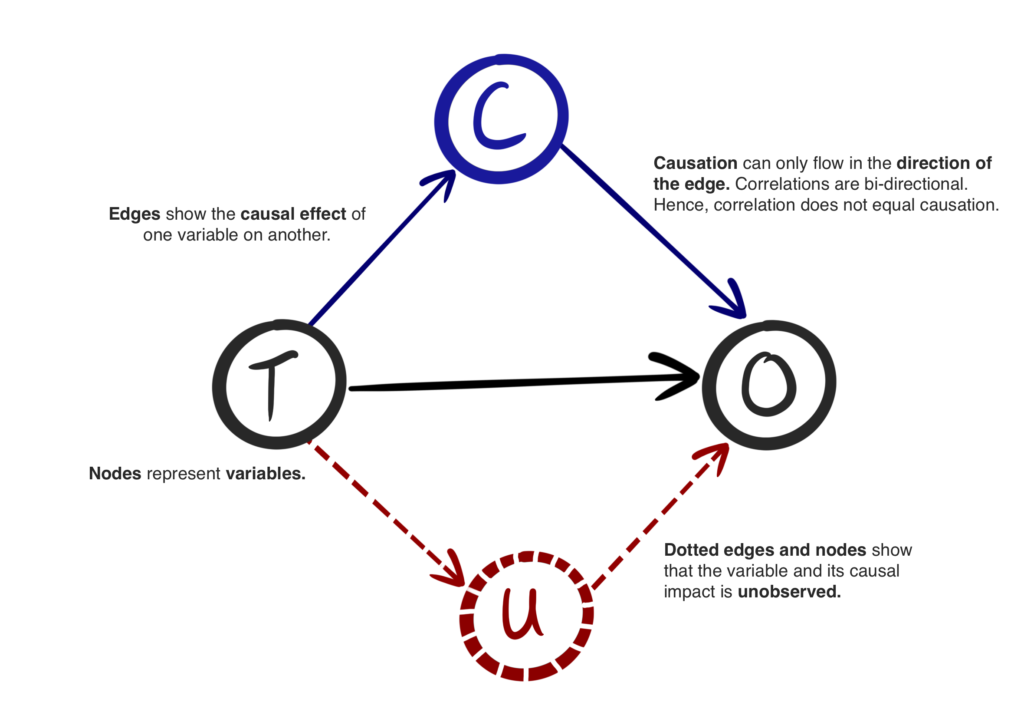
Causal Graph Image Source: Causalens
Measuring Average Treatment Effect (ATE)
The Average Treatment Effect (ATE) is a measure used to evaluate the average impact of a treatment across all participants in a study. It is calculated by comparing the outcomes of the treatment and control groups.
Calculating ATE
To calculate the ATE, follow these steps:
- Identify the Individual Treatment Effect (ITE) for each participant, which is the difference between their treatment and control outcomes.
- Sum the ITEs for all participants.
- Divide the sum by the total number of participants to get the ATE.
Example Calculation
Based on the data:
This example is from the video titled "Causal Inference - EXPLAINED!" available on YouTube.
| Participant | Age | Treatment Outcome | Control Outcome | Individual Treatment Effect (ITE) |
|---|---|---|---|---|
| Ajay | 26 | 1 | 1 | 0 |
| Sam | 24 | 0 | 1 | -1 |
| Less | 48 | 0 | 0 | 0 |
| Sid | 35 | 1 | 1 | 0 |
| Clay | 25 | 0 | 0 | 0 |
| Rhode | 39 | 1 | 0 | 1 |
| Clyde | 51 | 1 | 0 | 1 |
| Rondo | 24 | 0 | 1 | -1 |
| Chrom | 67 | 1 | 1 | 0 |
| Don | 34 | 1 | 0 | 1 |
ATE = (0 - 1 + 0 + 0 + 0 + 1 + 1 - 1 + 0 + 1) / 10 = 0.1
Conditional Average Treatment Effect (CATE)
The Conditional Average Treatment Effect (CATE) measures the average treatment effect for a specific subgroup of participants.
Example Calculation
For participants aged 35 and above:
- Less: ITE = 0
- Sid: ITE = 0
- Rhode: ITE = 1
- Clyde: ITE = 1
- Chrom: ITE = 0
CATE(age ≥ 35) = (0 + 0 + 1 + 1 + 0) / 5 = 0.4
For participants under 35:
- Ajay: ITE = 0
- Sam: ITE = -1
- Clay: ITE = 0
- Rondo: ITE = -1
- Don: ITE = 1
CATE(age < 35)=(0 - 1 + 0 - 1 + 1) / 5=-0.2
These calculations help determine the effectiveness of the treatment across different groups